Teaching an AI how to play the classic game Snake
22 Nov 2020
- Introduction
- Snake
- The Snake environment
- Training of the agent
- Using it to play the game
- Summary
- References
Introduction
In this article we are going to use reinforcement learning (RL) [1] to teach a computer to play the classic game Snake [2] (remember the good old Nokia phones?). The game is implemented from scratch using Python including a visualization with PySDL2 [3]. We are going to use TensorFlow [4] to implement the actor-critic algorithm [5] which is then used to learn playing the game.
We will show that, with moderate effort, an agent can be trained which plays the game reasonably well.
Figure 1: The agent playing the game on a 10x10 board for 500 steps.
Snake
Snake is a name for a series of video games where the player controls a growing “snake”-like line. According to Wikipedia the game concept is as old as 1976 and because it is so easy to implement (but still fun!) a ton of different implementations exist for nearly every computer platform. Many of you will probably know Snake from Nokia phones. Nokia started putting a variant of Snake onto their mobile phones in 1998, which brought a lot of new attention to this game. I, for myself, have to admit to have spent too much time trying to feed that little snake on my Nokia 6310.
The gameplay is simple: The player controls a dot, square, or something similar on a 2d world. As it moves, it leaves a tail behind, resembling a snake. Usually the length of the tail depends on the amount of food the snake ate. As the goal is to eat as much food as possible to increase your score, the length of the snake keeps increasing. The player loses when the snake runs into itself or into the screen border.
The game can easily be implemented in a few lines of Python code and when you throw in a couple more, you can even make a simple visualization in PySDL2. Therefore, we implemented the game ourselves, as relying on other implementations or looking into using them, may have taken more time than just doing it ourselves. And: It’s a fun little project to code.
We modified the traditional behavior of an automatically moving snake to a snake, which only moves one step when it gets the next action. This may make it boring if you are playing as a human, but it saves boilerplate code to discretize the game output into separate observations again. We believe, that the agent is fast enough to handle also that time constraint, if you should really want to use it in the self-moving game.
In our implementation always one piece of food is placed randomly onto an empty field of the game. The initial length of the snake is one tile, therefore, the maximum score for a given game field size of $N_x$ x $N_y$ is $N_xN_y - 1$.
The Snake environment
In addition to the game itself, it is necessary to encapsulate the game in an environment suitable for machine learning. We need to be able to tell the game what to do (which step to perform next) and we need a way to get an observation describing the current game state.
It is necessary to have four discrete actions to control the snake:
- Move up
- Move left
- Move down
- Move right
Determining the best state representation for our agent took more experimenting: The first approach was to encode all the tiles of the field with its type in a one-dimensional tensor. While this did work well, we soon found out, that this is not easily generalizable, because the observation space grows or shrinks with the size of the game board and one cannot just train one model and reuse it on other board sizes. Then we came up with a different idea: Restrict the snakes visibility range to a certain amount of tiles around its head. This helps reducing the state space dramatically, it speeds up the learning and it lifts the restriction to a fixed field size. We decided, arbitrarily, that we are going to restrict its view to four tiles in each of the possible movement directions (for an example see the blue tiles in Figure 2).
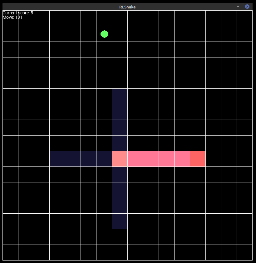
Figure 2: The agent playing the game on a 16x16 board. The tiles in the agents view are colored in blue.
For the rewards per step we first tried it with
- +10 when food was eaten
- -0.5 when no food was eaten
- -100 when game over (hitting a wall or itself)
which turned out to be a bad decision. Most of the time the agent just tried to stay on the same spot, being “afraid” of hitting a wall or itself, because that penalty was much larger than getting the slight penalty of not eating.
We then changed the rewards per step to
- +1 when food was eaten
- -0.01 when no food was eaten
- -1 when game over (hitting a wall or itself)
which worked reasonably well.
Training of the agent
After a bit of experimentation, we decided on a model with one hidden layer and 512 neurons. We were able to use a learning rate of $1e-3$ through the whole training without running into instabilities. The discount factor was set to $\gamma=0.995$. Usually we stopped playing an episode when the agent reached 200 steps. Then the episode would end without negative reward.
We trained the model in four phases: In the first run, we used a 4x4 field and ran for 100k episodes to see if the agent is improving. Next we continued training on the same field size for additional 500k episodes. Then we switched to a larger game field of 8x8 and trained for another 500k episodes. In the final training phase we increased the number of maximal steps for each episode to 400 and increased the field size to 10x10.
In Figure 3 the evolution of the total moves per episode is shown. The number of moves tend to go up to the maximum of 200/400, but with strong fluctuations for the first two training runs, which took place on small game field. The fluctuations reduce in the third training run, were we switched to the larger board. In the last training run a drop in the total moves can be observed after 155k episodes.
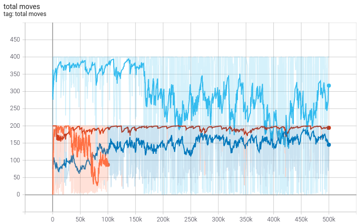
Figure 3: Total moves the agent reached during the episodes of training (note: the episode stopped automatically after 200 moves in the first 3 runs and after 400 moves in the last run). Plots taken from TensorBoard. The different colors of the lines correspond to the different phases of training: orange - first run, dark blue - second run, red - third run and light blue - final run. The data is smoothed using the TensorBoard smoothing value of 0.9.
The total reward per episode (Figure 4) shows a clear trend of improving during training. but also that training beyond a certain number of episodes does not increase the total rewards any further, due to the saturation on the small game field. Increasing the game field allowed a rise in the total rewards again. The final run, on an even larger field, seemed to show the same behavior up to about 155k episodes, but then a massive drop in total rewards could be observed.

Figure 4: Total reward the agent reached during the episodes of training. Plots taken from TensorBoard. The different colors of the lines correspond to the different phases of training: orange - first run, dark blue - second run, red - third run and light blue - final run.
The final plot shows the running reward over the course of the training (Figure 5). The running reward $R$ at episode $i$ is calculated as
\[R_{i} = 0.01R^{(e)}_i + 0.99 R_{i}\]where $R^{(e)}_i$ is the reward of the current episode $i$. Due to its definition its much smoother and a better indicator for the training progress of the model. The saturation due to limited field size is much clearer here and it seems to saturate between 11 and 12 for the 4x4 field, around 16 for the 8x8 field and around 21 for the 10x10 field. Judging from the fact, that the maximum score for the agent on a 4x4 field is 15 (taking into account the initial size of 1 tile for the snake), this is a good value, especially as our food placement is completely random and does not take into account if the food can be reached by the snake or not.

Figure 5: Running reward during training. Plots taken from TensorBoard. The different colors of the lines correspond to the different phases of training: orange - first run, dark blue - second run, red - third run and light blue - final run.
The most noticeable event happened during the fourth run. It seems we encountered the effect of catastrophic forgetting after approximately 150k episodes. Because of that we decided to take the model at the 150kth episode as the final model.
Using it to play the game
Already from the training it was clear that the agent learned to play the game quite well. It learned to cycle the game field and when it encounters food in its vision range it tries to catch it and it is taking into account that it is not allowed to move over its own tail.
Figure 6: A video of the agent playing snake on a 16x16 game field.
However, for larger game fields the agent can become stuck in a loop while searching for food, because if it cycles across the field without encountering food in his view, it will just continue cycling. But up to 16x16 boards, the agent works quite well.
Summary
We showed that for the simple game Snake a well working agent can be trained using the simple actor-critic algorithm with one hidden layer and 512 neurons. Once trained, the agent can play on different game field sizes from 4x4 up to 16x16 fields. Increasing the field sizes further, may lead to the agent getting stuck in a loop, depending on the (random) placement of the foods on the field.
Ways to improve the agent would be changing the view to not be just a cross, but a square, so that also food diagonally away from the agent can be seen. For larger fields an easy way to increase its efficiency is to increase the view range to values larger than the currently used four tiles in each direction. However, that will require longer training. Maybe a better solution can be found which lets the agent explore the field more efficiently.
Other ideas for continuing on that project would be to introduce more than one food on the field or walls inside the field. Both are easy to implement and, with enough training, the agent should be able to overcome these additional difficulties.
If you want to give it a try, the code is available on GitHub: https://github.com/torlenor/rlsnake
References
[1] https://en.wikipedia.org/wiki/Reinforcement_learning
[2] https://en.wikipedia.org/wiki/Snake_(video_game_genre)
[3] https://github.com/marcusva/py-sdl2
[4] https://www.tensorflow.org/
[5] A. Barto, R. Sutton, and C. Anderson, Neuron-like elements that can solve difficult learning control problems, IEEE Transactions on Systems, Man and Cybernetics, 13 (1983), pp. 835–846.