Ordinary least squares linear regression in Rust
29 Mar 2022
- Introduction
- Linear Regression
- Implementation in Rust
- Example: Diabetes dataset
- Summary
- Next steps
- References
Introduction
In contrast to the widespread use of Python and common machine learning packages like scikit-learn [1], there is an advantage in doing things from scratch. For example, learning how things work gives you an advantage in choosing the right algorithms for the job later down the line. We will start doing that with the simplest machine learning algorithm and maybe the most commonly used one: linear regression. In this article we are going to implement the so called ordinary least squares (OLS) [2] linear regression [3] in Rust [4]. We will show that with just a few lines of code it is possible to implement this algorithm from scratch. We will then work through an example and compare it with known results. During this work we will gain a better understanding of the concept behind the algorithm and we learn about the Rust package called nalgebra [5], which will help us with our linear algebra needs.
Linear Regression
What is linear regression
Linear regression [3] is used to model the relationship between a response/target variable and (multiple) explanatory variables or parameters. It is called linear, because the coefficients in the model are linear. A linear model for the target variable $y_i$ can be written in the form
\[y_i = \beta_{0} + \beta_{1} x_{i1} + \cdots + \beta_{p} x_{ip} + \varepsilon_i \, , \qquad i = 1, \ldots, n \; ,\]where $x_{ip}$ are the explanatory variables and $\beta_{p}$ are unknown coefficients. The $\varepsilon_i$ are called error terms or noise and they capture all the other information that we cannot explain with the linear model.
It is much easier to work with these equations if one writes them in matrix form as
\[\mathbf{y} = X\boldsymbol\beta + \boldsymbol\varepsilon \, ,\]where all the $n$ equations are squashed together. As we will see below, this notation is useful for deriving our method of determining the parameters $\boldsymbol\beta$. Note: Here we integrated the $\beta_0$ in the $\boldsymbol\beta$ and therefore $\boldsymbol\beta$ is now a $(p+1)$-dimensional vector and $\mathbf{X}$ is now a (n, p+1)-dimensional matrix, where we include a constant first column, i.e., $x_{i0}=1$ for $i = 1, \ldots, n$.
The goal is to get values for all the $\boldsymbol\beta$ fulfilling the equation above.
Solution of the equation
Ordinary least squares (OLS) [2] is, as the name suggests, a least squares method for find the unknown parameters $\boldsymbol\beta$ for a linear regression model. The idea is to minimize the sum of squares of the differences between the observed target variable and the predicted target variable coming from the linear regression model.
For the linear case the minimization problem possesses a unique global minimum and its solution can be expressed by an explicit formula for the coefficients $\boldsymbol\beta$:
\[\boldsymbol\beta = (\mathbf{X}^\mathbf{T}\mathbf{X})^{-1}\mathbf{X}^\mathbf{T}\mathbf{y}\]As we can see here, we have to calculate a matrix inverse and we have to make some assumptions on the input values to guarantee that the solution exists and the matrix is invertible. One of these assumptions is, for example, that the column vectors in $\mathbf{X}$ are linearly independent.
If you are interested in the derivation of this solution, please take a look at the linked Wikipedia page or any good statistics book.
Implementation in Rust
Finally, we are at the point where we can start implementing the algorithm. As it is basically given by some matrix/vector multiplications and inversions, we have two choices: either we implement the matrix/vector options ourselves or we use a library. As I want to focus on the algorithm implementation, I chose to use a library (nalgebra [5]).
Before we start, we need to bring in the nalgebra functions that we are going to use
extern crate nalgebra as na;
use std::ops::Mul;

use na::{DMatrix, DVector};
Then we define the x values and the y values that we want to fit
let x_training_values = na::dmatrix![
    1.0f64, 3.0f64;
    2.0f64, 1.0f64;
    3.0f64, 8.0f64;
];
let y_values = na::dvector![2.0f64, 3.0f64, 4.0f64];
As you can see, we use two x variables, which means we are going to have a model of the form
\[y = \beta_{0} + \beta_{1} x_{1} + \beta_{2} x_{2} \; ,\]Fitting the model can be performed as follows:
beta = x_values
    .tr_mul(&x_values)
    .try_inverse()
    .unwrap()
    .mul(x_values.transpose())
    .mul(y_values);
This also tries to calculate the inverse of the $X^TX$ matrix. As this can fail, if the matrix is not invertible (for example because the columns in $x$ are not linearly independent), in a production environment one should handle this gracefully and don’t use unwrap. For our coding example, however, it is good enough.
Getting predictions is then as simple as
let prediction = x_values.mul(beta);
The full source code for LinearRegression can be seen here (excuse the unwraps). It contains a bit more boilerplate, but also supports fitting without the intercept term, which can be useful if the data is already centered around its mean (in which case the intercept would be zero).
use std::ops::Mul;

use na::{DMatrix, DVector};

/// Ordinary least squares linear regression
///
/// It fits a linear model of the form y = b_0 + b_1*x + w_2*x_2 + ...
/// which minimizes the residual sum of squared between the observed targets
/// and the predicted targets.
pub struct LinearRegression {
    w: Option<DVector<f64>>,
    fit_intercept: bool,
}

impl LinearRegression {
    /// Returns a linear regressor using ordinary least squares linear regression
    ///
    /// # Arguments
    ///
    /// * `fit_intercept` - Whether to fit a intercept for this model.
    ///     If false assume that the data is centered, i.e., intercept is 0.
    ///
    pub fn new(fit_intercept: bool) -> LinearRegression {
        LinearRegression {
            w: None,
            fit_intercept,
        }
    }

    /// Fit the model
    ///
    /// # Arguments
    ///
    /// * `x_values` - parameters of shape (n_samples, n_features)
    /// * `y_values` - target values of shape (n_samples)
    pub fn fit(&mut self, x_values: &DMatrix<f64>, y_values: &DVector<f64>) {
        if self.fit_intercept {
            let x_values = x_values.clone().insert_column(0, 1.0);
            self._fit(&x_values, y_values);
        } else {
            self._fit(x_values, y_values);
        }
    }
    fn _fit(&mut self, x_values: &DMatrix<f64>, y_values: &DVector<f64>) {
        self.w = Some(
            x_values
                .tr_mul(&x_values)
                .try_inverse()
                .unwrap()
                .mul(x_values.transpose())
                .mul(y_values),
        );
    }
    pub fn coef(&self) -> &Option<DVector<f64>> {
        // TODO: Do not return 0th entry if fit_intercept is active
        return &self.w;
    }
    pub fn intercept(&self) -> Result<f64, String> {
        if !self.w.is_some() {
            return Err("Model was not fitted".to_string());
        }
        if self.fit_intercept {
            return Ok(self.w.as_ref().unwrap()[0]);
        }
        return Err("Model was not fitted with intercept".to_string());
    }

    /// Returns the predictions using the provided parameters `x_values`
    ///
    /// # Arguments
    ///
    /// * `x_values` - parameters of shape (n_samples, n_features)
    pub fn predict(&self, x_values: &DMatrix<f64>) -> Result<DVector<f64>, String> {
        if let Some(w) = self.w.as_ref() {
            if self.fit_intercept {
                let x_values = x_values.clone().insert_column(0, 1.0);
                let res = x_values.mul(w);
                return Ok(res);
            } else {
                let res = x_values.mul(w);
                return Ok(res);
            }
        }
        Err("Model was not fitted.".to_string())
    }
}
This is a crude version of this implementation and assumes fixed data types. For using it in a more convenient way, a bit more work has to be invested. If I decide to upload it to my GitHub page, I will update this blog post.
Example: Diabetes dataset
As an example we will follow the scikit-learn example about OLS. There they use a feature of the diabetes dataset [6] and perform linear regression on it. In addition, they calculate the mean squared error and the $R^2$ score. We will do the same and also try to fit the model using more features and see if it increases/decreases the score.
The first thing that we try it, is to take the full dataset (442 records, 10 feature variables $x$, standardized to have mean 0 and $\sum(x_i^2)=1$ and the last column is the variable that we want to predict) and try to fit it with our code.
We decide, as in the scikit-learn example, that we want to take bmi (3rd column in the dataset) as our feature variable and we want to predict y (the last column in the dataset). After reading them into an nalgebra matrix and vector, we can fit the model with
let mut model = LinearRegression::new(true);
model.fit(&x_values, &y_values);
where the parameter true indicates that we want to fit the intercept.
The result of the fit provides us with the model parameters
Coeffs: 949.435260383949
Intercept: 152.1334841628967
We can also calculate the scores based on the true values, which gives us
MSE of fit: 3890.456585461273
R^2 of fit: 0.3439237602253802
and we can plot the regression line as seen in Fig. 1.

Figure 1: Fit to the complete diabetes dataset. The purple circles indicate the true data points and the red line indicates the linear model.
We can also try it with additional features, let’s say taking not only the bmi, but also the cholesterol values ldl and hdl. For that model we get the scores
MSE of fit: 3669.2644919453955
R^2 of fit: 0.3812250059259711
which seems to be a slight improvement and the model seems to explain a bit more of the variance in the data.
As usually, you split the data into a training and a test set, we will do the same and follow exactly the scikit-learn example. This will serve as the final test! Can we reproduce the scikit-learn results with our code? In their example, they take the first 422 records as the training set and the last 20 records as the test set. We will do the same!
After reading the data and performing the split, we train our model again using the bmi. We find as the model parameters
Coeffs: 938.2378612512634
Intercept: 152.91886182616173
and as scores
MSE of fit: 2548.072398725972
R^2 of fit: 0.472575447982271
which is exactly as in the scikit-learn example. We can also reproduce the plot that they show (see Fig. 2).
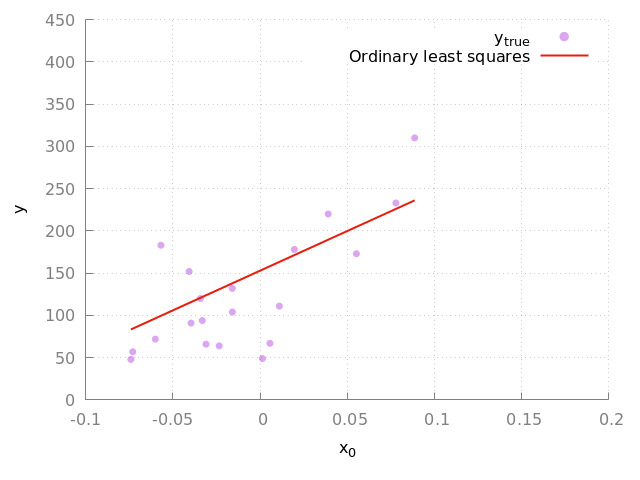
Figure 2: Fit to the complete diabetes dataset. The purple circles indicate the true data points and the red line indicates the linear model. Here we show the result of the validation data set.
So, we did it. We just implemented (I have to admit, a quite simple) machine learning algorithm ourselves and made sure that the results are exactly the same as in one of the most used Python libraries out there.
Summary
This concludes this brief excursion into linear regression and demonstrates, that some things are not that complicated as they seem and it may make sense to implement some of those algorithms from scratch to get a better understanding what they do and what’s behind all the magic.
Next steps
Possible next steps from here could be:
- Implementation of (stochastic) gradient descent linear regression
- Look into classification models (perceptron, k-nearest neighbors, logistic regression)
- Explore unsupervised methods, like support vector machines (SVMs)
References
[1] https://scikit-learn.org/stable/
[2] https://en.wikipedia.org/wiki/Ordinary_least_squares
[3] https://en.wikipedia.org/wiki/Linear_regression
[4] https://www.rust-lang.org/
[5] https://nalgebra.org/
[6] Bradley Efron, Trevor Hastie, Iain Johnstone and Robert Tibshirani (2004) “Least Angle Regression,” Annals of Statistics (with discussion), 407-499, https://www4.stat.ncsu.edu/~boos/var.select/diabetes.html